Neural Processing Elements
Note: The following text almost entirely coincides with parts of chapter 2 of my PhD thesis. I am republishing it here because I want to rework it in a more accessible form and because it is a good case study for the tooling needed to get a “nice” blogging setup.
The nervous system has besides its complicated dynamics a particular structure. The working hypothesis of connectionism is that how the primitive components used to model neurons are connected that is its structure already in large part determines the (potential) function. The question then becomes to what degree of fidelity the structure of the biological nervous system needs to be understood and captured in order to derive useful functional models. Arguably the most important characteristic of of biological nervous systems is their capability to “adapt” or “learn” beyond the innate function they had at birth.
In this article I describe a framework based on category theory, which allows for the description of self-optimizing “machines”, which I call “Neural Processing Elements”. Those machines can be composed and nested to form larger machines. The category theory perspective on “wiring diagrams” has been advanced in several papers [1–3]. In some ways the description I give here is just a different perspective on well known results in the literature, which I will point out along the way. Furthermore I will not actually give any formal defintions here. This would require the introduction of far more background material. Rather the ideas I present here informed my thinking on the problem of self-optimizing systems.
While I want to consider a more general case later, let me first discuss artificial neural networks. In the case of artificial neural networks advances in their computational power significantly derived from structural innovations. While it is well known that a two layer artificial neural network is in principle already capable of approximating a large class of functions, in practice restrictions on connectivity and parameter sharing as in convolutional architectures, residual neural networks [4], as well as transformer and attention architectures [5], demonstrate the large impact that choice of structures have.
Moreover choice of structure or network architecture both has an impact on the feasability of solving a given task, as well as the convergence speed of the training algorithm. A basic insight is that the choice of structure can already ensure that a network can be trained to accomplish a wide range of domain specific tasks (vision, natural language processing, etc.).
The main enabling innovation in the case of artificial neural networks is the backpropagation algorithm [6–8]. Briefly speaking it answers the question how to efficiently compute derivatives of a function composed out of a set of primitive functions with respect to parameters, in the case that the space of parameters has much higher dimensionality than the co-domain of the function. The basic insight is that this problem can be reduced to a two-phase message passing algorithm: By assumption the function can be computed by a directed acyclic graph whose nodes are primitives \phi and edges are variables. During the forward pass values are propagated along these edges to ultimately compute the function, while simultaneously the input values to each node (or more generally a context) is recorded. During the backward pass cotangent vectors are propagated and at each node the \phi^* with respect to the given primitive at the input computed during the forward pass is computed. While this algorithm lends itself well to bulk-synchronous parallel implementations (c.f. [9] and references therein) it exhibits inherent forward-backward locking in that the backward phase depends on values computed during the forward phase.
From a programming language perspective a curious feature of artificial neural network models is that their architecture can typically be described very concisely in terms of few repeating and nested primitives, together with task specific parameters. This enables the development of hardware accelerators, which then can focus on implementing this short list of primitives in an efficient manner. Furthermore to support gradient based training one can associate to each primitive a way to compute the between the output and input cotangent spaces, which in practice means that the number of supported operations has to be doubled. In other words operations come in pairs.
One such pair is addition and copying \begin{aligned} + &\colon \mathbf{R} \times \mathbf{R} \to \mathbf{R}, (x,y) \mapsto x + y, \\ \Delta &\colon \mathbf{R} \to \mathbf{R} \times \mathbf{R}, dz \mapsto (dz,dz) \end{aligned} another is multiplication m and an operation m^* \begin{aligned} m &\colon \mathbf{R} \times \mathbf{R} \to \mathbf{R}, (x,y) \mapsto x \cdot y, \\ m^* &\colon (\mathbf{R} \times \mathbf{R}) \times \mathbf{R} \to \mathbf{R} \times \mathbf{R}, ((x,y), dz) \mapsto (y \cdot dz, x \cdot dz). \end{aligned} Most generally to any smooth map between (pointed) manifolds f \colon (M, p) \to (N, f(p)) we can associate the map between cotangent spaces f^* \colon T^*_{f(p)} N \to T^*_p M. This turns out to be a functor.
We now want to associate to each of the primitives \phi a e(\phi) that computes \phi and to each of the pullback primitives \phi^* a e^* = e(\phi^*) that computes \phi^*. What is meant concretely by “processing element” depends on further details. Let us say for example we wanted to implement primitives as digital circuits. To implement an addition primitive + \colon \mathbf{R} \times \mathbf{R} \to \mathbf{R} for example a choice of value representation must be made, since digital circuits can’t operate on real numbers and there are then still multiple options to implement the control and datapath of a digital adder. Other primitives like matrix multiplication could in principle be regarded as being composed of elementary operations, but the most efficient implementation of the overall operation in realistic settings in many cases is not a composition of implementations of these more primitive operations. In many ways large parts of neumorphic engineering are concerned with coming up with novel ways of implementing matrix multiplication primitives in various physical inncarnations.
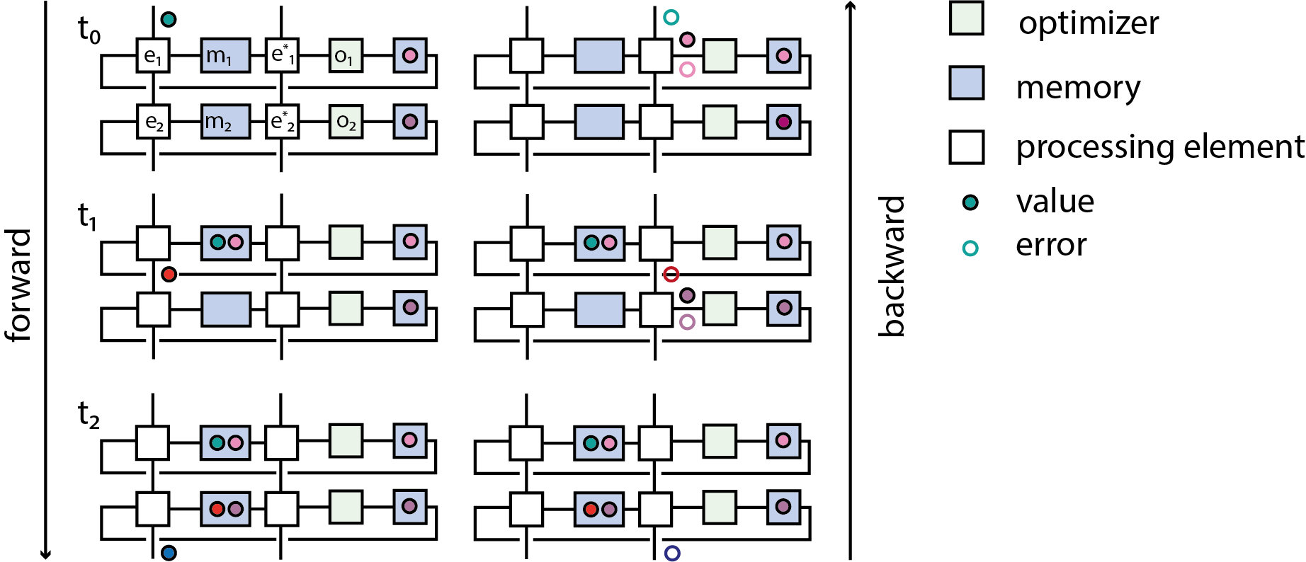
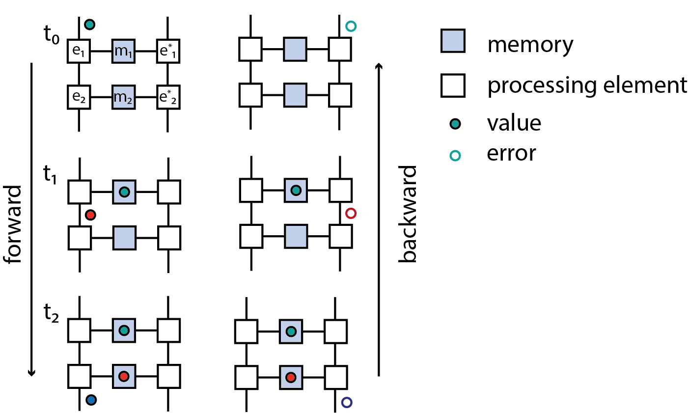
Once a choice of implementation is made we want to demand that there is a notion of composition of the implementation of primitives, which is compatible with the composition of the primitives. In the case of artificial neural network primitives this is illustrated in fig. . Each primitive is computed by a processing element, during the forward pass the input values need to be stored in a memory. Assuming the memory can hold only one value, the processing element has to be blocked until during the backward pass the computation of the pullback consumes the input value. As it turns out an analogous algorithm can be derived when each processing element operates in continuous time and operates either on events or continuous signals.
![Figure 2: Illustration of merging (A) and splitting of (B) implemented by processing elements. The merge processing element m_{k,l} implements the primitive \phi \colon \mathbf{R}^k \times \mathbf{R}^l \to \mathbf{R}^{k + l}, (x,y) \mapsto [x_1, \ldots, x_k, y_1, \ldots, y_l] and the element m^*_{l,k} implements the pullback \phi^* \colon \mathbf{R}^{k + l} \to \mathbf{R}^k \times \mathbf{R}^{l}, [x_1, \ldots, x_k, y_1, \ldots, y_l] \mapsto (x,y). Similarly the split processing element s_{k,l} implements the primitive \psi \colon \mathbf{R}^{k + l} \to \mathbf{R}^k \times \mathbf{R}^{l}, [x_1, \ldots, x_k, y_1, \ldots, y_l] \mapsto (x,y). and the element s^*_{l,k} implements the pullback \psi^* \colon \mathbf{R}^k \times \mathbf{R}^l \to \mathbf{R}^{k + l}, (x,y) \mapsto [x_1, \ldots, x_k, y_1, \ldots, y_l].](figures/pe_merge_split.png)
Informally what we are aiming for is a way of describing the hierachical composition of time-continuous or discrete time processes, which “learn” or self-optimise over time. We want to decompose the problem into two parts: A way to describe the structure of interconnected systems of elements, that is the legal “diagrams” without specifying their “dynamics” and then a way to associate a “function” or “dynamics” to a given diagram. These vague notions have been made precise in several instances by describing the “structure” of the system by a suitable operad and the “function” by an operad algebra [3]. There the brain is also explicitely mentioned as one example of a complex hierachically composed system. Running the program we sketched so far to completion would therefore mean to first desribe an operad of neural processing elements and then define an operad algebra which exhibits “self-optimization” or “learning”, where again these terms would need to be defined further.
In the context of artificial neural networks a category theoretic approach has been pursued by [10,11]. Without an emphasis on learning, various “networks” of components have been described in this framework as well (Event based systems [1] , hybrid systems [2], open dynamical systems [10,12–14]). In the context of physics such wiring diagrams were of course first considered by Feynman to describe probability amplitutes in quantum mechanics and later QED. Specifying Feynman rules corresponds to the specification of an operad algebra, indeed this algebraic view in the context of Feynman diagrams is well known [15,16].